Tutorial: Synchrotron and Synchrotron Self Compton

In this tutorial we will show how to compute the spectral energy distribution (SED) produced by the synchrotron and synchrotron Self-Compton radiative processes in a jetted AGN.

# import numpy, astropy and matplotlib for basic functionalities
import numpy as np
import astropy.units as u
from astropy.constants import m_e
from astropy.coordinates import Distance
import matplotlib.pyplot as plt
from IPython.display import Image

# import agnpy classes
from agnpy.spectra import PowerLaw
from agnpy.emission_regions import Blob
from agnpy.synchrotron import Synchrotron
from agnpy.compton import SynchrotronSelfCompton
from agnpy.utils.plot import plot_sed, load_mpl_rc

load_mpl_rc()

Emission Region

Let us consider that the emission region is a spherical plasmoid of radius \(R_b = 10^{16}\,\mathrm{cm}\), streaming with Lorentz factor \(\Gamma=10\) in the AGN jet, resulting in a Doppler boosting of \(\delta_D=10\) (the jet is almost aligned with the observer’s line of sight). The galaxy hosting the active nucleus is at a distance of \(d_L=10^{27}\,\mathrm{cm}\). The blob has a tangled magnetic field \(B=1\,\mathrm{G}\). The electron spectrum is described by a power law with index \(-2.8\) and a total energy content of \(W_e = 10^{48}\,{\rm erg}\).

# blob properties
R_b = 1e16 * u.cm
V_b = 4 / 3 * np.pi * R_b ** 3
z = Distance(1e27, unit=u.cm).z
delta_D = 10
Gamma = 10
B = 1 * u.G

# electron distribution
W_e = 1e48 * u.Unit("erg")

n_e = PowerLaw.from_total_energy(
    W=W_e, V=V_b, p=2.8, gamma_min=1e2, gamma_max=1e7, mass=m_e
)

blob = Blob(R_b, z, delta_D, Gamma, B, n_e=n_e)

# the blob object is printable, returning a summary of its properties
print(blob)

* Spherical emission region
 - R_b (radius of the blob): 1.00e+16 cm
 - t_var (variability time scale): 4.13e-01 d
 - V_b (volume of the blob): 4.19e+48 cm3
 - z (source redshift): 0.07 redshift
 - d_L (source luminosity distance):1.00e+27 cm
 - delta_D (blob Doppler factor): 1.00e+01
 - Gamma (blob Lorentz factor): 1.00e+01
 - Beta (blob relativistic velocity): 9.95e-01
 - theta_s (jet viewing angle): 5.74e+00 deg
 - B (magnetic field tangled to the jet): 1.00e+00 G
 - xi (coefficient for 1st order Fermi acceleration) : 1.00e+00
* electrons energy distribution
 - power law
 - k: 9.27e+06 1 / cm3
 - p: 2.80
 - gamma_min: 1.00e+02
 - gamma_max: 1.00e+07

# we can also print the total electrons number and energy
print(f"total particle number: {blob.N_e_tot:.2e}")
print(f"total energy in electrons: {blob.W_e:.2e}")

total particle number: 5.44e+51
total energy in electrons: 1.00e+48 erg

# as well as the jet power in particles and magnetic fields (see the documentation for more details)
print(f"jet power in particles: {blob.P_jet_ke:.2e}")
print(f"jet power in magnetic field: {blob.P_jet_B:.2e}")

jet power in particles: 4.47e+44 erg / s
jet power in magnetic field: 7.46e+43 erg / s

Synchrotron Radiation

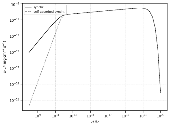
To intitialise the object that will compute the synchrotron radiation, we simply pass the Blob instance to the Synchrotron class. The synchrotron self absorption can be considered when computing the SED.

synch = Synchrotron(blob)
synch_ssa = Synchrotron(blob, ssa=True)

# let us define now a grid of frequencies over which to calculate the synchrotron SED
nu_syn = np.logspace(8, 23) * u.Hz

# let us compute a synchrotron, and a self-absorbed synchrotron SED
synch_sed = synch.sed_flux(nu_syn)
synch_sed_ssa = synch_ssa.sed_flux(nu_syn)

fig, ax = plt.subplots(figsize=(8, 6))
plot_sed(nu_syn, synch_sed, ax=ax, color="k", label="synchr.")
plot_sed(
    nu_syn, synch_sed_ssa, ax=ax, ls="--", color="gray", label="self absorbed synchr."
)
plt.show()

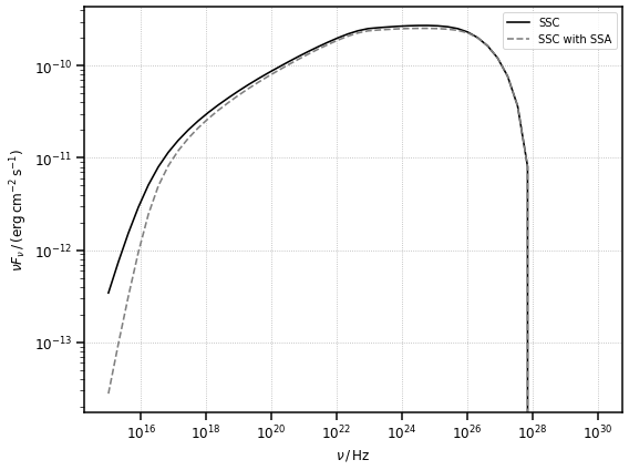
Synchrotron Self-Compton Radiation

Similarly to the synchrotron case, to intitialise the object that will compute the synchrotron self-Compton (SSC) radiation, we simply pass the Blob instance to the SynchrotronSelfCompton class.

We examine also the case produced by scattering over a self-absorbed synchrotron spectrum.

# simple ssc
ssc = SynchrotronSelfCompton(blob)

# ssc over a self-absorbed synchrotron spectrum
ssc_ssa = SynchrotronSelfCompton(blob, ssa=True)

nu_ssc = np.logspace(15, 30) * u.Hz
sed_ssc = ssc.sed_flux(nu_ssc)
sed_ssc_ssa = ssc_ssa.sed_flux(nu_ssc)

/Users/cosimo/work/agnpy/agnpy/synchrotron/synchrotron.py:66: RuntimeWarning: divide by zero encountered in true_divide
  u = 1 / 2 + np.exp(-tau) / tau - (1 - np.exp(-tau)) / np.power(tau, 2)
/Users/cosimo/work/agnpy/agnpy/synchrotron/synchrotron.py:66: RuntimeWarning: invalid value encountered in true_divide
  u = 1 / 2 + np.exp(-tau) / tau - (1 - np.exp(-tau)) / np.power(tau, 2)

fig, ax = plt.subplots(figsize=(8, 6))

plot_sed(nu_ssc, sed_ssc, color="k", label="SSC")
plot_sed(nu_ssc, sed_ssc_ssa, ls="--", color="gray", label="SSC with SSA")
plt.show()

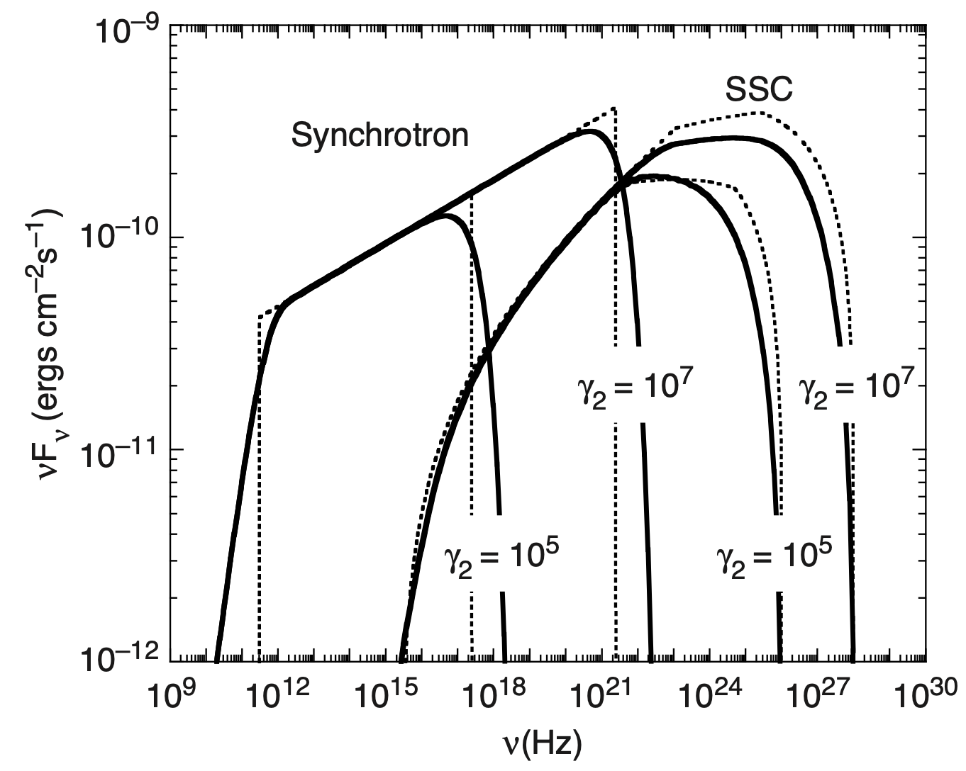
Literature Check from Dermer and Menon (2009)

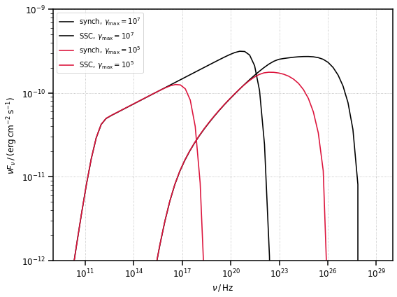
In order to provide a cross-check with the literature, we reproduce Figure 7.4 of Dermer and Menon (2009) - see bibliography in the docs. The figure, reported here, depicts two complete synchrotron and SSC SEDs, generated by the same emission regions distinguished only by the different maximum Lorentz factor of their electron distributions (\(\gamma_{\rm max} = 10^5\) and \(\gamma_{\rm max} = 10^7\)).

Image("figures/figure_7_4_dermer_2009.png", width=600, height=400)

The Blob previosuly defined is already set with the parameters reproducing the example with \(\gamma_{\rm max} = 10^7\), let us create a new Blob containing an electron distribution with \(\gamma_{\rm max} = 10^5\).

n_e = PowerLaw.from_total_energy(
    W=W_e, V=V_b, p=2.8, gamma_min=1e2, gamma_max=1e5, mass=m_e
)

blob2 = Blob(R_b, z, delta_D, Gamma, B, n_e=n_e)
synch2 = Synchrotron(blob2)
ssc2 = SynchrotronSelfCompton(blob2)

fig, ax = plt.subplots(figsize=(8, 6))

plot_sed(
    nu_syn,
    synch.sed_flux(nu_syn),
    color="k",
    label=r"${\rm synch},\,\gamma_{\rm max}=10^7$",
)
plot_sed(
    nu_ssc,
    ssc.sed_flux(nu_ssc),
    color="k",
    label=r"${\rm SSC},\,\gamma_{\rm max}=10^7$",
)
plot_sed(
    nu_syn,
    synch2.sed_flux(nu_syn),
    color="crimson",
    label=r"${\rm synch},\,\gamma_{\rm max}=10^5$",
)
plot_sed(
    nu_ssc,
    ssc2.sed_flux(nu_ssc),
    color="crimson",
    label=r"${\rm SSC},\,\gamma_{\rm max}=10^5$",
)

# select the same x and y range of the figure
plt.xlim([1e9, 1e30])
plt.ylim([1e-12, 1e-9])
plt.show()