Inverse Compton
Two different Compton processes are considered:
synchrotron self Compton (SSC), implemented in
SynchrotronSelfCompton, considering as target for the inverse Compton the synchrotron photons produced in the blob by the accelerated electrons (based on [DermerMenon2009] and [Finke2008]);external Compton (EC), implemented in
ExternalCompton, considering as a target for the inverse Compton the (direct and reprocessed) photon fields generated by the accretion phenomena (based on [Dermer2009] and [Finke2016]).
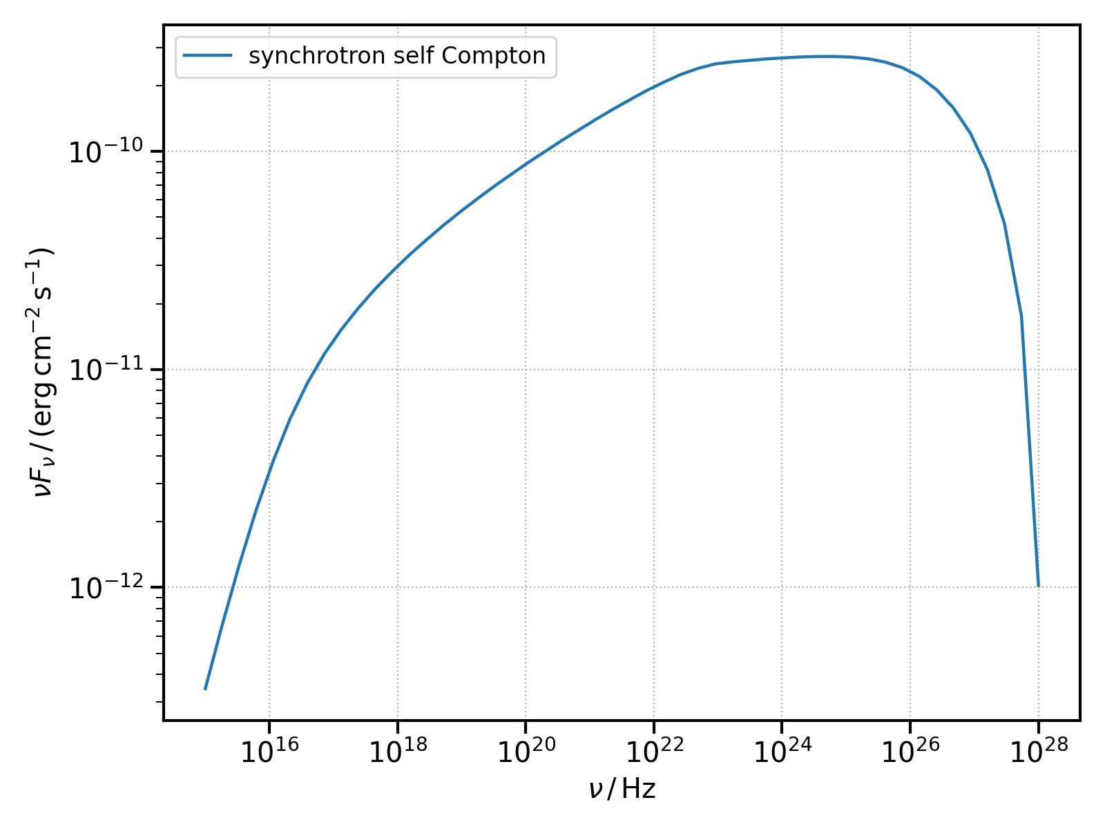
Synchrotron Self Compton
The synchrotron self Compton radiation calculation works exactly as the Synchrotron Radiation one.
The instance of the emission region has to be passed to the radiative class initialiser.
SED can be evaluated over an array of frequencies with the sed_flux method.
import numpy as np
import astropy.units as u
from astropy.constants import m_e
from astropy.coordinates import Distance
from agnpy.spectra import PowerLaw
from agnpy.emission_regions import Blob
from agnpy.compton import SynchrotronSelfCompton
from agnpy.utils.plot import plot_sed, load_mpl_rc
import matplotlib.pyplot as plt


# set the quantities defining the blob
R_b = 1e16 * u.cm
V_b = 4 / 3 * np.pi * R_b ** 3
z = Distance(1e27, unit=u.cm).z
delta_D = 10
Gamma = 10
B = 1 * u.G

# electron distribution
W_e = 1e48 * u.erg # total energy in electrons

n_e = PowerLaw.from_total_energy(
    W_e,
    V_b,
    p=2.8,
    gamma_min=1e2,
    gamma_max=1e7,
    mass=m_e,
)

# define the emission region and the radiative process
blob = Blob(R_b, z, delta_D, Gamma, B, n_e=n_e)
ssc = SynchrotronSelfCompton(blob)

# compute the SED over an array of frequencies
nu = np.logspace(15, 28) * u.Hz
sed = ssc.sed_flux(nu)

# plot it
load_mpl_rc()
plot_sed(nu, sed, label="synchrotron self Compton")

plt.show()
(Source code, png, hires.png, pdf)

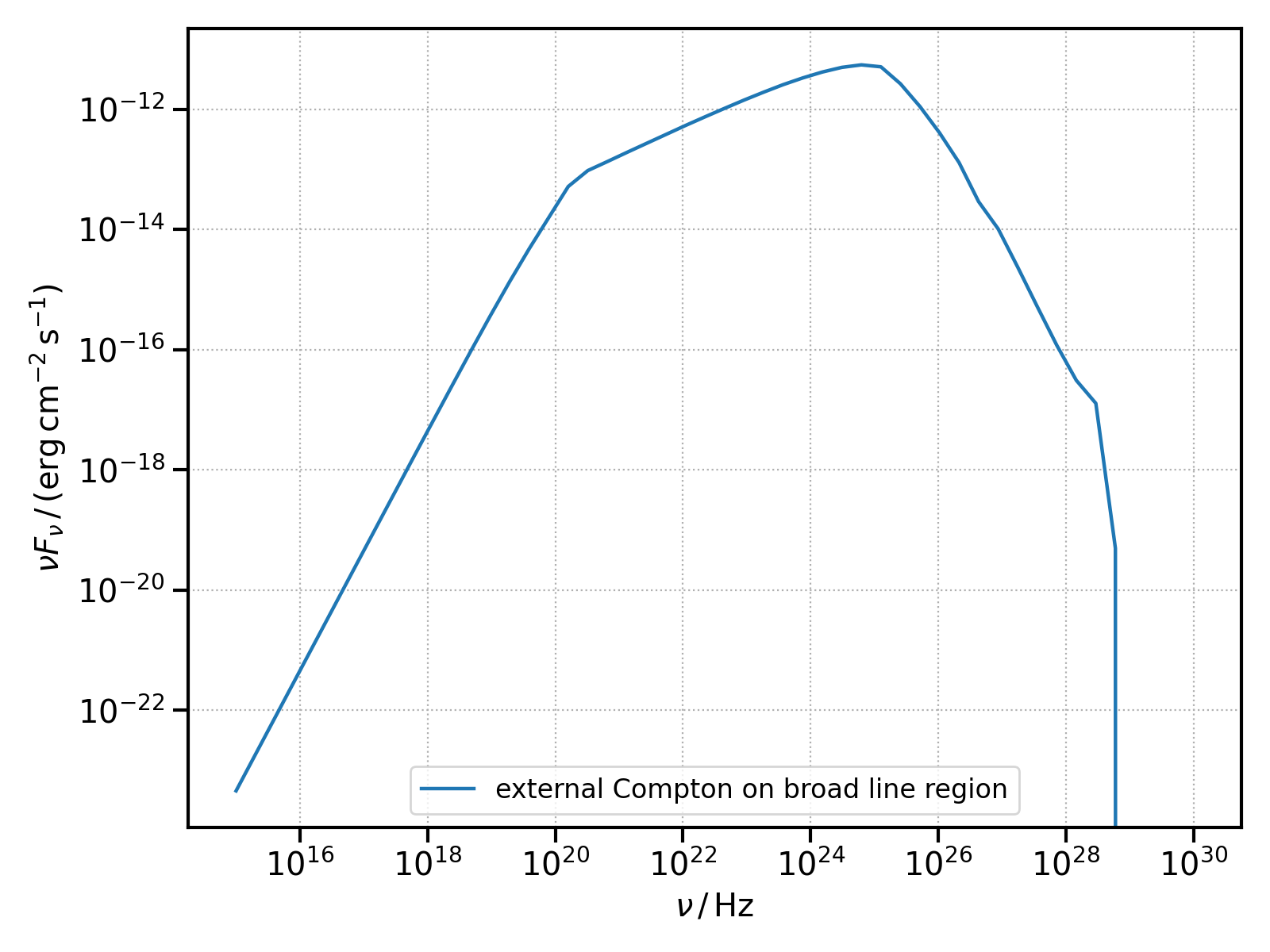
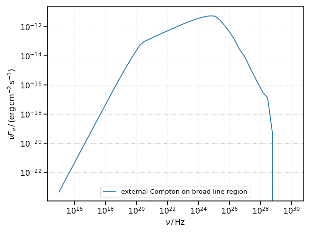
External Compton
As an example of this process, let us consider Compton scattering of the photon field produced by the broad line region by a power-law electron distribution.
import numpy as np
import astropy.units as u
from astropy.constants import m_e
from agnpy.spectra import BrokenPowerLaw
from agnpy.emission_regions import Blob
from agnpy.compton import ExternalCompton
from agnpy.targets import SphericalShellBLR
from agnpy.utils.plot import plot_sed
import matplotlib.pyplot as plt
from agnpy.utils.plot import load_mpl_rc


# define the emission region and the electron distribution
R_b = 1e16 * u.cm
V_b = 4 / 3 * np.pi * R_b ** 3
z = 1
delta_D = 40
Gamma = 40
B = 0.56 * u.G

W_e = 6e45 * u.erg
n_e = BrokenPowerLaw.from_total_energy(
    W=W_e, V=V_b, p1=2.0, p2=3.5, gamma_b=1e4, gamma_min=20, gamma_max=5e7, mass=m_e
)

blob = Blob(R_b, z, delta_D, Gamma, B, n_e, gamma_e_size=500)


# define the target
L_disk = 2 * 1e46 * u.Unit("erg s-1")
xi_line = 0.024
R_line = 1e17 * u.cm

blr = SphericalShellBLR(L_disk, xi_line, "Lyalpha", R_line)


# declare the external Compton process
# distance between the blob and the target
r = 2e17 * u.cm
ec = ExternalCompton(blob, blr, r)

# compute the SED over an array of frequencies
nu = np.logspace(15, 30) * u.Hz
sed = ec.sed_flux(nu)

# plot it
load_mpl_rc()
plot_sed(nu, sed, label="external Compton on broad line region")

plt.show()
(Source code, png, hires.png, pdf)
As we can see from the snippet, the EC radiation can be computed passing to the ExternalCompton
class
the instance of the emission region (
Blob);the instance of the target (
SphericalShellBLR);the distance between the blob and the target photon field (
r).
You can use any object in the targets module as target for external Compton.
For more examples of Inverse Compton radiation and reproduction of literature results,
check the tutorial notebook on external Compton.