Synchrotron Radiation

The synchrotron radiation is computed following the approach of [DermerMenon2009] and [Finke2008]. To compute the single-particle synchrotron power, the appoximation of [Aharonian2010] (Eq. D7) is used.

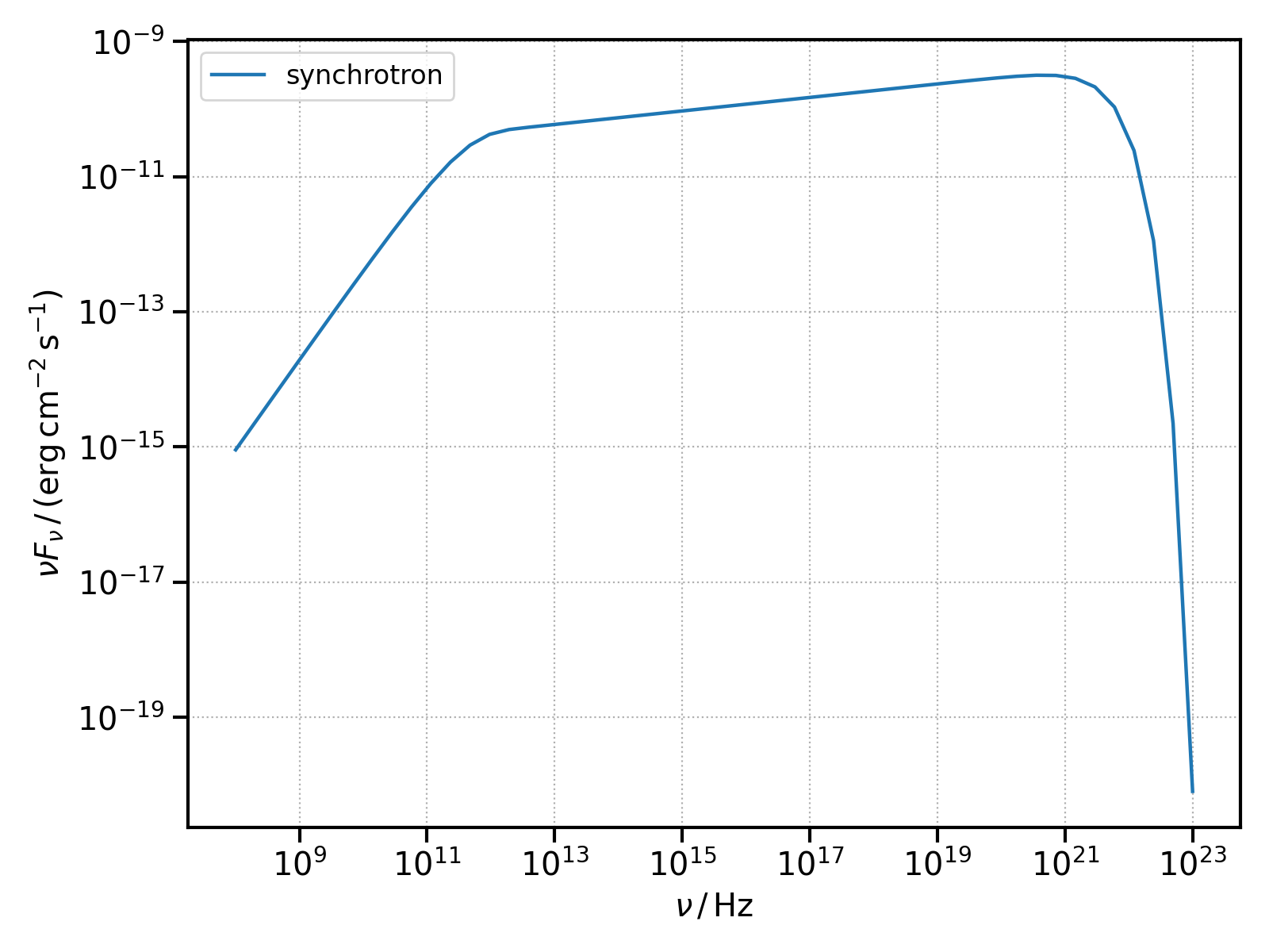
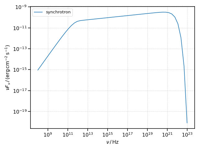
It is here illustrated how to produce a synchrotron spectral energy distribution (SED) staring from a Blob.

import numpy as np
import astropy.units as u
from astropy.constants import m_e
from astropy.coordinates import Distance
from agnpy.spectra import PowerLaw
from agnpy.emission_regions import Blob
from agnpy.synchrotron import Synchrotron
from agnpy.utils.plot import load_mpl_rc, plot_sed
import matplotlib.pyplot as plt


# set the quantities defining the blob
R_b = 1e16 * u.cm
V_b = 4 / 3 * np.pi * R_b ** 3
z = Distance(1e27, unit=u.cm).z
delta_D = 10
Gamma = 10
B = 1 * u.G

# electron distribution
W_e = 1e48 * u.erg # total energy in electrons

n_e = PowerLaw.from_total_energy(
    W_e,
    V_b,
    p=2.8,
    gamma_min=1e2,
    gamma_max=1e7,
    mass=m_e,
)

# define the emission region and the radiative process
blob = Blob(R_b, z, delta_D, Gamma, B, n_e=n_e)
synch = Synchrotron(blob)

# compute the SED over an array of frequencies
nu = np.logspace(8, 23) * u.Hz
sed = synch.sed_flux(nu)

# load matplotlib configuration for agnpy
load_mpl_rc()

plot_sed(nu, sed, label="synchrotron")
plt.show()

(Source code, png, hires.png, pdf)

Note two aspects valid for all the radiative processes in agnpy:

1. to initialise any radiative process in agnpy, the instance of the emission region class (Blob in this case) has to be passed to the initialiser of the radiative process class (Synchrotron in this case)

synch = Synchrotron(blob)

2. the SEDs are always compute over an array of frequencies (astropy units), passed to the sed_flux function

nu = np.logspace(8, 23) * u.Hz
sed = synch.sed_flux(nu)

this produces an array of Quantity.

For more examples of Synchrotron radiation and cross-checks of literature results, check the check the tutorial notebook on synchrotron and sycnrotron self Compton.