Absorption by \(\gamma\gamma\) pair production
The photon fields that provide the targets for the Compton scattering might re-asbsorb the scattered photons via
\(\gamma\gamma\) pair production. Similarly, on their path towards Earth, the highest-energy photons might be
absorbed by the extragalactic background light (EBL).
agnpy computes the optical depth (or opacity) \(\tau_{\gamma \gamma}\) as a function of the frequency \(\nu\)
produced by the AGN line and thermal emitters and by the EBL.
Photon absorption results in an attenuation of the flux by a factor \(\exp(-\tau_{\gamma \gamma})\).
Absorption calculation on line and thermal emitters
The \(\gamma\gamma\) absorption for a photon field with specific energy density \(u(\epsilon, \mu, \phi; l)\) reads:
- where:
\(\cos\psi = \mu\mu_s + \sqrt{1 - \mu^2}\sqrt{1 - \mu_s^2} \cos\phi\) is the cosine of the angle between the hitting and the absorbing photon;
\(u(\epsilon, \mu, \phi; l)\) is the energy density of the target photon field with \(\epsilon\) dimensionless energy, \((\mu, \phi)\) angles, \(l\) distance of the blob from the photon field;
\(\sigma_{\gamma \gamma}(s)\) is the pair-production cross section, with \(s = \epsilon_1 \epsilon \, (1 - \cos\psi)\,/\,2\) and \(\epsilon_1 = h \nu\,/\,(m_e c^2)\) the dimensionless energy of the hitting photon.
We employed the notation [Finke2016]. The approach presented therein (and in [Dermer2009]) simplifies the
integration by assuming that the hitting photons travels in the direction parallel to the jet axis (\(\mu_s \rightarrow 1\)),
decoupling the cross section and the \((1 - \cos\psi)\) term from the integral in \(\phi\).
The optical depths thus calculated are therefore valid only for blazars. agnpy instead allows to consider an
arbitrary viewing angle can be used. Optical depths thus obtained are valid for any jetted AGN.
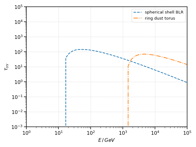
Absorption on target photon fields
In the following example we compute the optical depth produced by the the broad line region and the dust torus photon fields.
The Absorption requires as input:
the type of
targets;the distance between the blob and the target photon field (\(r\));
the redshift of the source to correct the observed energies.
import numpy as np
import astropy.units as u
from agnpy.targets import SphericalShellBLR, RingDustTorus
from agnpy.absorption import Absorption
import matplotlib.pyplot as plt
from agnpy.utils.plot import load_mpl_rc


# blr definition
L_disk = 2 * 1e46 * u.Unit("erg s-1")
csi_line = 0.024
R_line = 1e17 * u.cm
blr = SphericalShellBLR(L_disk, csi_line, "Lyalpha", R_line)

# dust torus definition
T_dt = 1e3 * u.K
csi_dt = 0.1
dt = RingDustTorus(L_disk, csi_dt, T_dt)

# consider a fixed distance of the blob from the target fields
r = 1.1e16 * u.cm
# let us consider 3C 454.3 as source
z = 0.859

absorption_blr = Absorption(blr, r=r, z=z)
absorption_dt = Absorption(dt, r=r, z=z)

# plot using the same energy range as in Finke 2016
E = np.logspace(0, 5) * u.GeV
nu = E.to("Hz", equivalencies=u.spectral())

tau_blr = absorption_blr.tau(nu)
tau_dt = absorption_dt.tau(nu)

# plot it
load_mpl_rc()
plt.loglog(E, tau_blr, lw=2, ls="--", label="spherical shell BLR")
plt.loglog(E, tau_dt, lw=2, ls="-.", label="ring dust torus")
plt.legend()
plt.xlabel(r"$E\,/\,GeV$")
plt.ylabel(r"$\tau_{\gamma \gamma}$")
plt.xlim([1, 1e5])
plt.ylim([1e-3, 1e5])
plt.show()
(Source code, png, hires.png, pdf)

For more examples of absorption calculation, especially for cases of “misaligned” sources, i.e. \(\mu_s \neq 1\), check the tutorial notebook on Absorption.
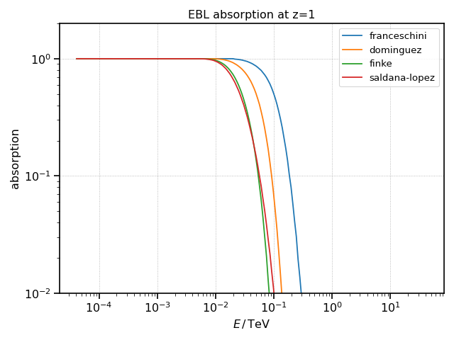
Extragalactic Background Light
The \(\gamma\gamma\) absorption produced by the EBL models of [Franceschini2008], [Franceschini2017], [Finke2010], [Dominguez2011] and [Saldana-Lopez2021], is available in data/ebl_models.
The absorption values, tabulated as a function of redshift and energy, are interpolated by agnpy and can be later evaluated for a given redshift and range of frequencies.
# check absorption for different EBL model at redshift z=1
import numpy as np
import astropy.units as u
from agnpy.absorption import EBL
import matplotlib.pyplot as plt
from agnpy.utils.plot import load_mpl_rc

load_mpl_rc()

# redshift and array of frequencies over which to evaluate the absorption
z = 0.5
nu = np.logspace(22, 28, 200) * u.Hz
E = nu.to("TeV", equivalencies=u.spectral())

for model in ["franceschini_2008", "franceschini_2017", "dominguez_2011", "finke_2010", "saldana_lopez_2021"]:
    ebl = EBL(model)
    absorption = ebl.absorption(
        nu, z
    )  # warning: in agnpy <= v0.4.0 the arguments order is reversed!
    plt.loglog(E, absorption, label=model.replace("_", " ").title())

plt.xlabel(r"$E\,/\,{\rm TeV}$")
plt.title(f"EBL absorption at z={z}")
plt.ylabel("absorption")
plt.ylim([1e-3, 2])
plt.legend()
plt.show()
(Source code, png, hires.png, pdf)