Non-thermal Particle Energy Distributions

The agnpy.spectra module provides classes describing the energy distributions of particles accelerated in the jets. The energy distribution is commonly represented by an analytical function, usually a power law, returning the volume density of particles, \(n [{\rm cm}]^{-3}\), as a function of their Lorentz factor, \(\gamma\). The following analytical functions are available:

Additionaly, an InterpolatedDistribution is available to interpolate an array of densities and Lorentz factors. This might be useful if you have obtained an electron distribution from another software (e.g. performing the time evolution of the particles distribution accounting for acceleration and energy losses) and want to use this result in agnpy.

Since v0.3.0, agnpy includes both electrons and protons energy distributions.

We can initialise a particle distribution specifying directly the parameters of the analytical function and the mass of the particle, for example:

import astropy.units as u
from astropy.constants import m_e, m_p
from agnpy.spectra import PowerLaw, BrokenPowerLaw
import matplotlib.pyplot as plt

# electron distribution
n_e = BrokenPowerLaw(
    k=1e-8 * u.Unit("cm-3"),
    p1=1.9,
    p2=2.6,
    gamma_b=1e4,
    gamma_min=10,
    gamma_max=1e6,
    mass=m_e,
)

# proton distribution
n_p = PowerLaw(k=0.1 * u.Unit("cm-3"), p=2.3, gamma_min=10, gamma_max=1e6, mass=m_p)

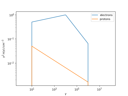
# let us plot both particle distributions
fig, ax = plt.subplots()

n_e.plot(ax=ax, gamma_power=2, label="electrons")
n_p.plot(ax=ax, gamma_power=2, label="protons")

ax.legend()
plt.show()

(Source code, png, hires.png, pdf)

Different ways to initialise (or normalise) the particle energy distribution

Authors use different approaches to define the particles distribution \(n(\gamma)\). A normalisation of the distribution is often provided, which can be of different types.

Some authors use an integral normalisation. That is, the normalisation value provided might represent:

the total volume density, \(n_{\rm tot} = \int {\rm d \gamma} \, n(\gamma)\), in \({\rm cm}^{-3}\);
the total energy density, \(u_{\rm tot} = \int {\rm d \gamma} \, \gamma \, n(\gamma)\), in \({\rm erg}\,{\rm cm}^{-3}\);
the total energy in particles, \(W = m c^2 \, \int {\rm d \gamma} \, \gamma \, n(\gamma)\), in \({\rm erg}\).

Others use a differential normalisation, that is, the normalisation value provided directly represents the constant, \(k\), multiplying the analytical function, e.g. for a power law

\[n(\gamma) = k \, \gamma^{-p}.\]

Finally, some authors use a normalisation at \(\gamma=1\), that means the normalisation value provided represents the value of the denisty at \(\gamma=1\).

We offer all of the aforementioned alternatives to initialise a particles distribution in agnpy. Here follows an example illustrating them:

import numpy as np
import astropy.units as u
from astropy.constants import m_e
from agnpy.spectra import LogParabola
import matplotlib.pyplot as plt

# initialise the electron distribution, let us use the same spectral parameters
# for all the distributions
p = 2.3
q = 0.2
gamma_0 = 1e3
gamma_min = 1
gamma_max = 1e6

# - from total density
n_tot = 1e-3 * u.Unit("cm-3")

n_1 = LogParabola.from_total_density(
    n_tot, p=p, q=q, gamma_0=gamma_0, gamma_min=gamma_min, gamma_max=gamma_max, mass=m_e
)

# - from total energy density
u_tot = 1e-8 * u.Unit("erg cm-3")

n_2 = LogParabola.from_total_energy_density(
    u_tot, p=p, q=q, gamma_0=gamma_0, gamma_min=gamma_min, gamma_max=gamma_max, mass=m_e
)

# - from total energy, we need also the volume to convert to an energy density
W = 1e40 * u.erg
V_b = 4 / 3 * np.pi * (1e16 * u.cm) ** 3

n_3 = LogParabola.from_total_energy(
    W,
    V_b,
    p=p,
    q=q,
    gamma_0=gamma_0,
    gamma_min=gamma_min,
    gamma_max=gamma_max,
    mass=m_e,
)

# - from the denisty at gamma = 1
n_gamma_1 = 1e-4 * u.Unit("cm-3")

n_4 = LogParabola.from_density_at_gamma_1(
    n_gamma_1,
    p=p,
    q=q,
    gamma_0=gamma_0,
    gamma_min=gamma_min,
    gamma_max=gamma_max,
    mass=m_e,
)

# let us plot all the particles distributions
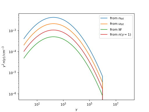
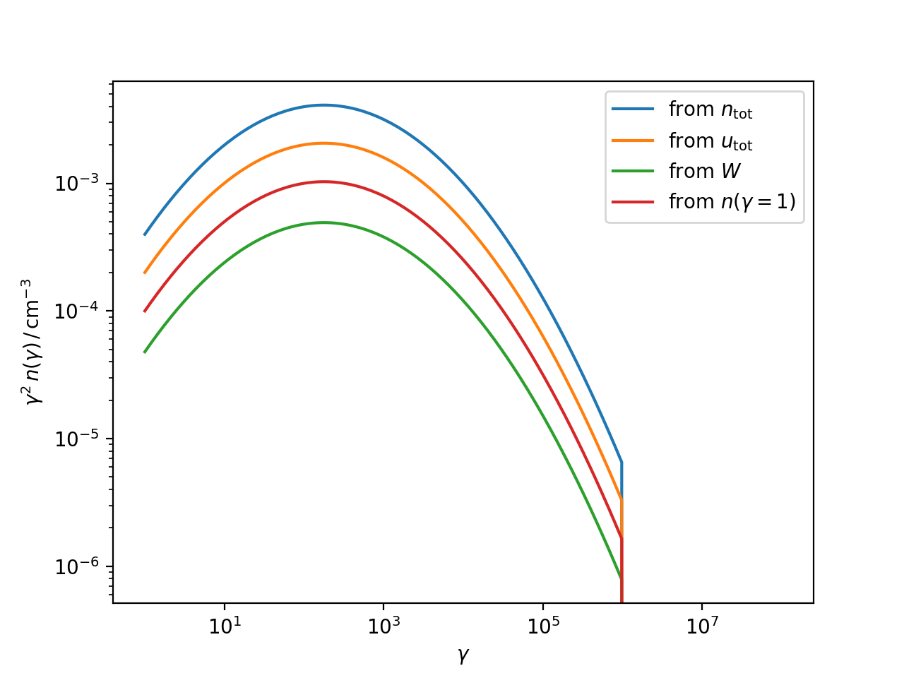
fig, ax = plt.subplots()

n_1.plot(ax=ax, gamma_power=2, label="from " + r"$n_{\rm tot}$")
n_2.plot(ax=ax, gamma_power=2, label="from " + r"$u_{\rm tot}$")
n_3.plot(ax=ax, gamma_power=2, label="from " + r"$W$")
n_4.plot(ax=ax, gamma_power=2, label="from " + r"$n(\gamma=1)$")

ax.legend()
plt.show()

(Source code, png, hires.png, pdf)