Tutorial: fitting a BL Lac broad-band SED using MCMC fit with Gammapy

In this tutorial, we will perform again the fit of the MWL SED of Mrk421 illustrated in this notebook. This time, instead of the simple $\chi^2$ minimisation with iminuit, we will perform a fit with a Monte Carlo Markov Chain (MCMC) method. As for the case of the simple $\chi^2$ minimisation, we will rely on Gammapy’s functionalities for data handling and fitting.

Some Gammapy functions wrapping the MCMC package, emcee, are available in the gammapy-recipes. Please download the gammapy-recipes repository to run the code in this notebook.

An excellent theoretical introduction to MCMC methods can be found in these notes.

[1]:

# import numpy, astropy and matplotlib for basic functionalities
import numpy as np
import astropy.units as u
import matplotlib.pyplot as plt
import pkg_resources

# import agnpy classes
from agnpy.spectra import BrokenPowerLaw
from agnpy.fit import SynchrotronSelfComptonModel, load_gammapy_flux_points
from agnpy.utils.plot import load_mpl_rc, sed_y_label

load_mpl_rc()

# import gammapy classes
from gammapy.modeling.models import SkyModel
from gammapy.modeling import Fit

[2]:

# the run_mcmc method has been moved from gammapy/gammapy to gammapy/recipes
# please download the gammapy-recipes
# https://github.com/gammapy/gammapy-recipes
# and change the following path accordingly
import sys

sys.path.append("/Users/cosimo/work/gammapy-recipes/recipes/mcmc-sampling-emcee")
from sampling import (
    run_mcmc,
    par_to_model,
    plot_corner,
    plot_trace,
)

`gammapy` wrapper of agnpy synchrotron and SSC

Please refer to the this notebook for a description of the Gammapy wrapper of the synchrotron and SSC radiative processes.

[3]:

# electron energy distribution
n_e = BrokenPowerLaw(
    k=1.3e-8 * u.Unit("cm-3"),
    p1=2.02,
    p2=3.43,
    gamma_b=1e5,
    gamma_min=500,
    gamma_max=1e6,
)

# initialise the Gammapy SpectralModel
ssc_model = SynchrotronSelfComptonModel(n_e, backend="gammapy")

[4]:

# set intial parameters
ssc_model.parameters["z"].value = 0.0308
ssc_model.parameters["delta_D"].value = 18
ssc_model.parameters["t_var"].value = (1 * u.d).to_value("s")
ssc_model.parameters["t_var"].frozen = True
ssc_model.parameters["log10_B"].value = -1.3

[5]:

ssc_model.parameters.to_table()

[5]:

Table length=11

type	name	value	unit	error	min	max	frozen	is_norm	link
str8	str15	float64	str1	int64	float64	float64	bool	bool	str1
spectral	log10_k	-7.8861e+00		0.000e+00	-1.000e+01	1.000e+01	False	False
spectral	p1	2.0200e+00		0.000e+00	1.000e+00	5.000e+00	False	False
spectral	p2	3.4300e+00		0.000e+00	1.000e+00	5.000e+00	False	False
spectral	log10_gamma_b	5.0000e+00		0.000e+00	2.000e+00	6.000e+00	False	False
spectral	log10_gamma_min	2.6990e+00		0.000e+00	0.000e+00	4.000e+00	True	False
spectral	log10_gamma_max	6.0000e+00		0.000e+00	4.000e+00	8.000e+00	True	False
spectral	z	3.0800e-02		0.000e+00	1.000e-03	1.000e+01	True	False
spectral	delta_D	1.8000e+01		0.000e+00	1.000e+00	1.000e+02	False	False
spectral	log10_B	-1.3000e+00		0.000e+00	-4.000e+00	2.000e+00	False	False
spectral	t_var	8.6400e+04	s	0.000e+00	1.000e+01	3.142e+07	True	False
spectral	norm	1.0000e+00		0.000e+00	1.000e-01	1.000e+01	True	True

Fit with `gammapy`

Here we start the procedure to fit with Gammapy.

1) load the MWL flux points and add the systematics

As in the previous example, we define a FluxPointsDataset for each instrument. We then proceed to add systematic errors using a very rough and conservative estimate ($30\%$ of the flux for VHE points, $10\%$ for HE and X-ray points, $5\%$ on all the other instruments data).

[6]:

sed_path = pkg_resources.resource_filename("agnpy", "data/mwl_seds/Mrk421_2011.ecsv")

systematics_dict = {
    "Fermi": 0.10,
    "GASP": 0.05,
    "GRT": 0.05,
    "MAGIC": 0.30,
    "MITSuME": 0.05,
    "Medicina": 0.05,
    "Metsahovi": 0.05,
    "NewMexicoSkies": 0.05,
    "Noto": 0.05,
    "OAGH": 0.05,
    "OVRO": 0.05,
    "RATAN": 0.05,
    "ROVOR": 0.05,
    "RXTE/PCA": 0.10,
    "SMA": 0.05,
    "Swift/BAT": 0.10,
    "Swift/UVOT": 0.05,
    "Swift/XRT": 0.10,
    "VLBA(BK150)": 0.05,
    "VLBA(BP143)": 0.05,
    "VLBA(MOJAVE)": 0.05,
    "VLBA_core(BP143)": 0.05,
    "VLBA_core(MOJAVE)": 0.05,
    "WIRO": 0.05,
}

# define minimum and maximum energy to be used in the fit
E_min = (1e11 * u.Hz).to("eV", equivalencies=u.spectral())
E_max = 100 * u.TeV

datasets = load_gammapy_flux_points(sed_path, E_min, E_max, systematics_dict)

No reference model set for FluxMaps. Assuming point source with E^-2 spectrum.
No reference model set for FluxMaps. Assuming point source with E^-2 spectrum.
No reference model set for FluxMaps. Assuming point source with E^-2 spectrum.
No reference model set for FluxMaps. Assuming point source with E^-2 spectrum.
No reference model set for FluxMaps. Assuming point source with E^-2 spectrum.
No reference model set for FluxMaps. Assuming point source with E^-2 spectrum.
No reference model set for FluxMaps. Assuming point source with E^-2 spectrum.
No reference model set for FluxMaps. Assuming point source with E^-2 spectrum.
No reference model set for FluxMaps. Assuming point source with E^-2 spectrum.
No reference model set for FluxMaps. Assuming point source with E^-2 spectrum.
No reference model set for FluxMaps. Assuming point source with E^-2 spectrum.
No reference model set for FluxMaps. Assuming point source with E^-2 spectrum.
No reference model set for FluxMaps. Assuming point source with E^-2 spectrum.
No reference model set for FluxMaps. Assuming point source with E^-2 spectrum.
No reference model set for FluxMaps. Assuming point source with E^-2 spectrum.
No reference model set for FluxMaps. Assuming point source with E^-2 spectrum.
No reference model set for FluxMaps. Assuming point source with E^-2 spectrum.
No reference model set for FluxMaps. Assuming point source with E^-2 spectrum.
No reference model set for FluxMaps. Assuming point source with E^-2 spectrum.
No reference model set for FluxMaps. Assuming point source with E^-2 spectrum.
No reference model set for FluxMaps. Assuming point source with E^-2 spectrum.
No reference model set for FluxMaps. Assuming point source with E^-2 spectrum.
No reference model set for FluxMaps. Assuming point source with E^-2 spectrum.
No reference model set for FluxMaps. Assuming point source with E^-2 spectrum.

[7]:

# define the model for this list of datasets
sky_model = SkyModel(spectral_model=ssc_model, name="Mrk421")
datasets.models = [sky_model]

2) run the fit

We define here the parameters for the MCMC fit and run it with the run_mcmc function in the gammapy recipes. nwalkers indicate the number of chains we want to use, a good rule is to use $n_{\rm walkers} \geq 2 \times n_{\rm free\;parameters}$. In this case we choose a number of walkers three times the number of free parameters (6, in this case). nrun indicates the number of steps of MCMC we want to perform. With the current settings, it will take roughly 1 hour, you can decrease one of the two parameters for testing purposes.

[8]:

%%time
sampler = run_mcmc(datasets, nwalkers=18, nrun=400)

CPU times: user 1h 16min 56s, sys: 8min 56s, total: 1h 25min 52s
Wall time: 1h 26min 8s

[9]:

plot_trace(sampler, datasets)

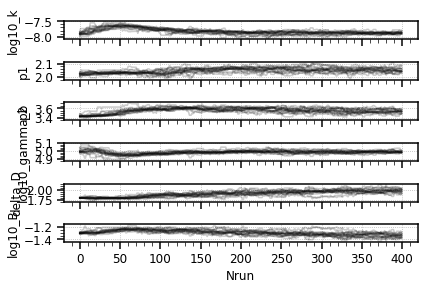
../_images/tutorials_ssc_gammapy_mcmc_fit_12_0.png

The figure above shows the trace, i.e. the position of each walker as a function of the number of steps in the chain. One can estimate the burn-in period, i.e. the time needed for the walkers to reach a stationary stage. To make this estimate more precise, take a look at emcee’s autocorrelation and analysis and convergence tutorial. For the sake of this example, and since it takes already a while to run this notebook, we will assume that after 300 steps the walkers are already “burnt in”.

[10]:

plot_corner(sampler, datasets, nburn=300)

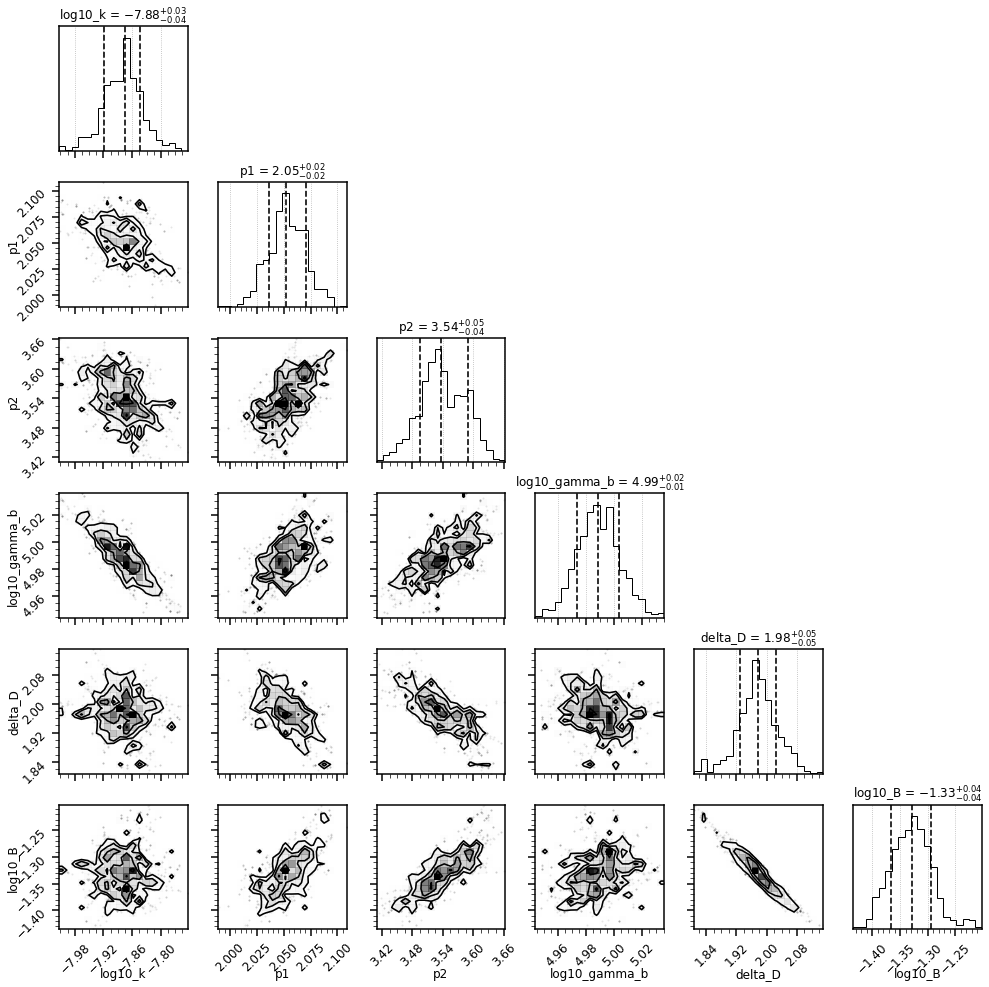
../_images/tutorials_ssc_gammapy_mcmc_fit_14_0.png

The figure above represents a corner plot. It shows different marginalisations of the total posterior distribution. Note that in this case, by default, a flat prior was used, spanning the interval we set through the min and max of each parameter.

The diagonal panels with the single histograms show the 1-D marginalised posterior distribution for each parameter, along with the corresponding median and 68% credible interval. They represent an estimate of the parameters and their errors. Each panel containing a 2-D histograms shows the the 2-D marginalized posterior distribution, along with the 16, 50 and 84% containment fraction. They illustrate the correlation between the different parameters.

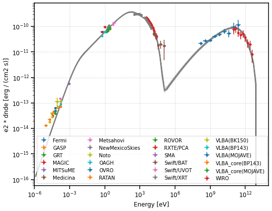
3) plot the results

To assess the results of our fit we can choose a small sample of parameters from the chain, and plot the corresponding models. We choose to plot the models corresponding to the last ten realisation of each walker.

[11]:

emin, emax = [1e-6, 1e14] * u.eV

fig, ax = plt.subplots(figsize=(8, 6))

for dataset in datasets:
    dataset.data.plot(ax=ax, label=dataset.name)


for nwalk in range(0, 18):
    for n in range(390, 400):
        pars = sampler.chain[nwalk, n, :]

        # set model parameters
        par_to_model(datasets, pars)

        ssc_model.plot(
            energy_bounds=(emin, emax),
            ax=ax,
            energy_power=2,
            alpha=0.02,
            color="grey",
            yunits=u.Unit("erg cm-2 s-1"),
        )

plt.legend(ncol=4)
plt.xlim([1e-6, 1e14])
plt.show()

../_images/tutorials_ssc_gammapy_mcmc_fit_16_0.png

Which values should we use for the final parameters and their uncertainty? The `emcee documentation <https://emcee.readthedocs.io/en/stable/tutorials/line/#results>`__ suggests to quote the uncertainties based on the 16th, 50th, and 84th percentiles of the samples in the marginalized distributions.

[12]:

from IPython.display import display, Math

for i, par in enumerate(
    [
        "\log_{10}(k_{\mathrm e}\,/\,{\mathrm cm}^{-3})",
        "p_1",
        "p_2",
        "\log_{10}(\gamma_{\mathrm b})",
        "\delta_{\mathrm D}",
        "\log_{10}(B\,/\,{\mathrm G})",
    ]
):

    # the sampler.chain has shape (# walker, # steps, # parameters)
    par_values = sampler.chain[:, 300:, i].flatten()
    mcmc = np.quantile(par_values, [0.16, 0.50, 0.84])
    q = np.diff(mcmc)

    txt = "{3} = {0:.2f}_{{-{1:.2f}}}^{{+{2:.2f}}}"
    txt = txt.format(mcmc[1], q[0], q[1], par)
    display(Math(txt))

$\displaystyle \log_{10}(k_{\mathrm e}\,/\,{\mathrm cm}^{-3}) = -7.88_{-0.04}^{+0.03}$

$\displaystyle p_1 = 2.05_{-0.02}^{+0.02}$

$\displaystyle p_2 = 3.54_{-0.04}^{+0.05}$

$\displaystyle \log_{10}(\gamma_{\mathrm b}) = 4.99_{-0.01}^{+0.02}$

$\displaystyle \delta_{\mathrm D} = 1.98_{-0.05}^{+0.05}$

$\displaystyle \log_{10}(B\,/\,{\mathrm G}) = -1.33_{-0.04}^{+0.04}$

We can observe a very nice agreement with the parameters values and errors obtained with the simple $\chi^2$ minimisation in the previous tutorial.