Tutorial: \(\gamma\gamma\) Absorption in the Photon Fields of Line and Thermal Emitters
In this tutorial we will illustrate how to use agnpy to compute the \(\gamma\gamma\) absorption due to the photon fields produced by the BLR and DT photon fields.
[1]:
import numpy as np
import astropy.units as u
from astropy.constants import M_sun
from astropy.coordinates import Distance
import matplotlib.pyplot as plt
[2]:
from agnpy.targets import SphericalShellBLR, RingDustTorus, PointSourceBehindJet
from agnpy.absorption import Absorption
from agnpy.utils.plot import load_mpl_rc

# matplotlib adjustments
load_mpl_rc()
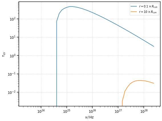
Absorption in the photon field of a spehrical shell BLR
Let us consider a BLR composed of a single spherical shell emitting the Ly\(\alpha\) line. Let us take, following Finke (2016) (see bibliography in the docs), the following parameters representing the blazar 3C 454.3: \(L_{\rm disk} = 2 \times 10^{46}\,{\rm erg}\,{\rm s}^{-1}\), \(\xi_{\rm li} = 0.1\), \(R_{\rm Ly\alpha} = 1.1 \times 10^{17}\,{\rm cm}\). The redshift of the source is \(z = 0.859\).
[3]:
L_disk = 2 * 1e46 * u.Unit("erg s-1")
xi_line = 0.1
R_line = 1.1 * 1e17 * u.cm
blr = SphericalShellBLR(L_disk, xi_line, "Lyalpha", R_line)
The Absorption class needs, to be initialised: the target instance, the distance from the target \(r\) and the redshift of the source (energies have to be converted to the galaxy frame). Let us actually compare the absorptions for two cases: inside (\(r = 0.1 \times R_{\rm Ly\alpha}\)) and outside (\(r = 10 \times R_{\rm Ly\alpha}\)) the BLR.
[4]:
z = 0.859
r_in_blr = 0.1 * R_line
r_out_blr = 10 * R_line

# evaluate the two absorptions
abs_in_blr = Absorption(blr, r=r_in_blr, z=z)
abs_out_blr = Absorption(blr, r=r_out_blr, z=z)
Let us evaluate the absorption in the same energy range considered in Figure 14 of Finke 2016: \([1, 10^5]\,{\rm GeV}\)
[5]:
E = np.logspace(0, 5) * u.GeV
nu = E.to("Hz", equivalencies=u.spectral())
# evaluate the opacities
tau_in_blr = abs_in_blr.tau(nu)
tau_out_blr = abs_out_blr.tau(nu)
/Users/cosimo/software/miniconda3/envs/gammapy-0.20.1/lib/python3.8/site-packages/astropy/units/quantity.py:613: RuntimeWarning: divide by zero encountered in true_divide
  result = super().__array_ufunc__(function, method, *arrays, **kwargs)
/Users/cosimo/software/miniconda3/envs/gammapy-0.20.1/lib/python3.8/site-packages/astropy/units/quantity.py:613: RuntimeWarning: invalid value encountered in sqrt
  result = super().__array_ufunc__(function, method, *arrays, **kwargs)
[6]:
# let us plot them
fig, ax = plt.subplots(figsize=(8, 6))

ax.loglog(nu, tau_in_blr, label=r"$r = 0.1 \times R_{\rm Ly\alpha}$")
ax.loglog(nu, tau_out_blr, label=r"$r = 10 \times R_{\rm Ly\alpha}$")
ax.legend()
ax.set_xlabel(r"$\nu\,/\,{\rm Hz}$", fontsize=12)
ax.set_ylabel(r"$\tau_{\gamma \gamma}$", fontsize=12)
plt.show()
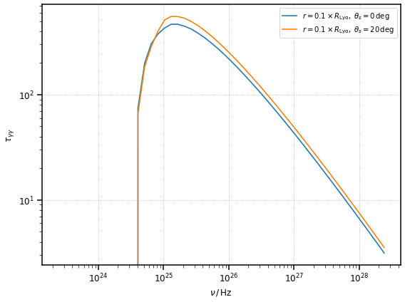
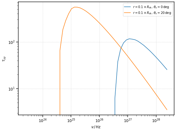
Opacity of a misaligned (non-blazar) source
In the default opacity calculation, agnpy assumes the line of sight of the observer to be aligned with the jet (i.e. the source is a blazar with \(\mu_s = 1\), where \(\theta_s\) is the viewing angle and \(\mu_s\) its cosine). This brings a considerable simplification in the opacity calculation (see the main documentation).
For some sources agnpy allows the calculation of the opacity for an aribitrary viewing angle (this is possible for BLR, DT and point source behind the blob). Let us assume we are considering a source with the same parameters of 3C 454.3 in the previous example, but with a viewing angle of \(20\,{\rm deg}\). Let us evaluate the absorption within the BLR for the aligned and misaligned case
[7]:
mu_s = np.cos(np.deg2rad(20))
abs_in_blr_mis = Absorption(blr, r=r_in_blr, z=z, mu_s=mu_s)
# evaluate the opacity
tau_in_blr_mis = abs_in_blr_mis.tau(nu)
[8]:
fig, ax = plt.subplots(figsize=(8, 6))

# compare the opacity in the aligned and misaligned case
ax.loglog(
    nu, tau_in_blr, label=r"$r = 0.1 \times R_{\rm Ly\alpha},\;\theta_s=0\,{\rm deg}$"
)
ax.loglog(
    nu,
    tau_in_blr_mis,
    label=r"$r = 0.1 \times R_{\rm Ly\alpha},\;\theta_s=20\,{\rm deg}$",
)
ax.legend()
ax.set_xlabel(r"$\nu\,/\,{\rm Hz}$", fontsize=12)
ax.set_ylabel(r"$\tau_{\gamma \gamma}$", fontsize=12)

plt.show()
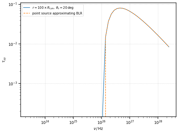
Comparison of the misaligned case with a point source behind the blob
The opacity for the misaligned case, in the limit of large distances, \(r >> R_{\rm Ly\alpha}\), should reduce to the same opacity produced by a monochromatic point source behind the jet approximating the BLR (in luminosity and emitted energy).
Note this comparison is not possible for the aligned case since for \(\mu_s=1\) there is no absorption from the target photons (factor \((1 - \mu_s)\) null in the opacity formula).
[9]:
# point source with the same luminosity as the BLR
ps_blr = PointSourceBehindJet(blr.xi_line * L_disk, blr.epsilon_line)

# absorption in the limit of very large distances
r_far_blr = 1e2 * R_line
abs_far_blr_mis = Absorption(blr, r=r_far_blr, z=z, mu_s=mu_s)
abs_far_ps_blr_mis = Absorption(ps_blr, r=r_far_blr, z=z, mu_s=mu_s)
[10]:
# compute the opacities
tau_far_blr_mis = abs_far_blr_mis.tau(nu)
tau_far_ps_blr_mis = abs_far_ps_blr_mis.tau(nu)
[11]:
fig, ax = plt.subplots(figsize=(8, 6))

# compare the opacity in the aligned and misaligned case
ax.loglog(
    nu,
    tau_far_blr_mis,
    label=r"$r = 100 \times R_{\rm Ly\alpha},\;\theta_s=20\,{\rm deg}$",
)
ax.loglog(nu, tau_far_ps_blr_mis, ls="--", label="point source approximating BLR")
ax.legend()
ax.set_xlabel(r"$\nu\,/\,{\rm Hz}$", fontsize=12)
ax.set_ylabel(r"$\tau_{\gamma \gamma}$", fontsize=12)

plt.show()
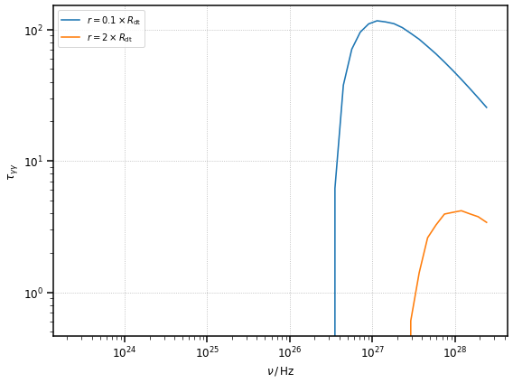
Absorption in the photon field of a ring dust torus
Let us consider a ring dust torus. Following Finke (2016) (see bibliography in the docs), we adopt the following parameters: \(L_{\rm disk} = 2 \times 10^{46}\,{\rm erg}\,{\rm s}^{-1}\), \(\xi_{\rm li} = 0.2\), \(T_{\rm dt} = 10^3\,{\rm K}\). The redshift of the source is \(z = 0.859\).
[12]:
dt = RingDustTorus(L_disk, 0.2, 1000 * u.K)
print(dt.R_dt)
1.565247584249853e+19 cm
Again, let us consider two cases of abosrption: inside (\(r = 0.1 \times R_{\rm dt}\)) and outside (\(r = 2 \times R_{\rm dt}\)) the torus
[13]:
r_in_dt = 0.1 * dt.R_dt
r_out_dt = 2 * dt.R_dt

# define the absorption objects
abs_in_dt = Absorption(dt, r=r_in_dt, z=z)
abs_out_dt = Absorption(dt, r=r_out_dt, z=z)

# evaluate the opacities
tau_in_dt = abs_in_dt.tau(nu)
tau_out_dt = abs_out_dt.tau(nu)
[14]:
fig, ax = plt.subplots(figsize=(8, 6))

# let us plot them
ax.loglog(nu, tau_in_dt, label=r"$r = 0.1 \times R_{\rm dt}$")
ax.loglog(nu, tau_out_dt, label=r"$r = 2 \times R_{\rm dt}$")
ax.legend()
ax.set_xlabel(r"$\nu\,/\,{\rm Hz}$", fontsize=12)
ax.set_ylabel(r"$\tau_{\gamma \gamma}$", fontsize=12)

plt.show()
Opacity of a misaligned (non-blazar) source
As already explained in the previous opacity calculation, agnpy will assume the line of sight of the observer to be aligned with the jet (\(\mu_s = 1\)). Let us perform a comparison with a source with the same dust torus defined above, but with a viewing angle of \(20\,{\rm deg}\). Let us evaluate the absorption within the DT for the aligned and misaligned case
[15]:
mu_s = np.cos(np.deg2rad(20))
abs_in_dt_mis = Absorption(dt, r=r_in_dt, z=z, mu_s=mu_s)
# evaluate the opacity
tau_in_dt_mis = abs_in_blr_mis.tau(nu)
[16]:
fig, ax = plt.subplots(figsize=(8, 6))

# compare the opacity in the aligned and misaligned case
ax.loglog(nu, tau_in_dt, label=r"$r = 0.1 \times R_{\rm dt},\;\theta_s=0\,{\rm deg}$")
ax.loglog(
    nu, tau_in_dt_mis, label=r"$r = 0.1 \times R_{\rm dt},\;\theta_s=20\,{\rm deg}$"
)
ax.legend()
ax.set_xlabel(r"$\nu\,/\,{\rm Hz}$", fontsize=12)
ax.set_ylabel(r"$\tau_{\gamma \gamma}$", fontsize=12)

plt.show()
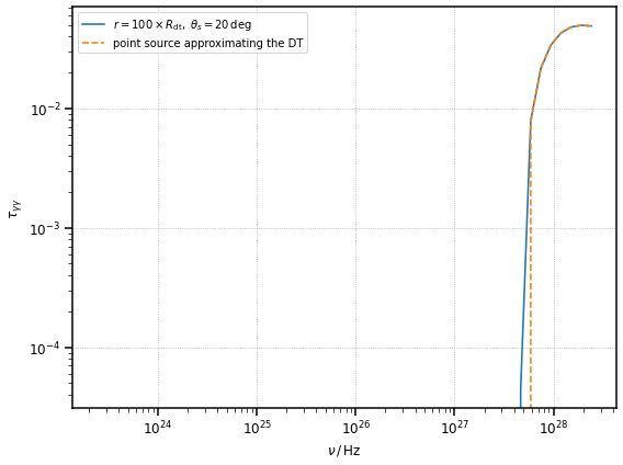
Comparison of the misaligned case with a point source behind the blob
And again, we can compare the opacity for the misaligned case, in the limit of large distances, \(r >> R_{\rm dt}\), with the opacity produced by a point source behind the jet approximating (in luminosity and emitted energy) the DT.
[17]:
# point source approximating the dust torus
ps_dt = PointSourceBehindJet(dt.xi_dt * L_disk, dt.epsilon_dt)

# absorption in the limit of very large distances
r_far_dt = 100 * dt.R_dt
abs_far_dt_mis = Absorption(dt, r=r_far_dt, z=z, mu_s=mu_s)
abs_far_ps_dt_mis = Absorption(ps_dt, r=r_far_dt, z=z, mu_s=mu_s)
[18]:
# compute the opacities
tau_far_dt_mis = abs_far_dt_mis.tau(nu)
tau_far_ps_dt_mis = abs_far_ps_dt_mis.tau(nu)
[19]:
fig, ax = plt.subplots(figsize=(8, 6))

# compare the opacity in the aligned and misaligned case
ax.loglog(
    nu, tau_far_dt_mis, label=r"$r = 100 \times R_{\rm dt},\;\theta_s=20\,{\rm deg}$"
)
ax.loglog(nu, tau_far_ps_dt_mis, ls="--", label="point source approximating the DT")
ax.legend()
ax.set_xlabel(r"$\nu\,/\,{\rm Hz}$", fontsize=12)
ax.set_ylabel(r"$\tau_{\gamma \gamma}$", fontsize=12)

plt.show()