Time evolution

Radiative models implemented in agnpy are primarily intended to compute radiation in a steady state. The time evolution module extends this functionality by enabling time-dependent modelling. The evaluation logic can be described by the following algorithm:

Choose an array of energies covering the blob’s particle spectrum range (an array of gamma values).
For all gamma values, create narrow energy bins and compute the corresponding particle density in each bin.
Calculate energy change rates at the start and end points of each bin.
Multiply the energy change rates by the time step duration.
Compute the new bin energy and the new particle density for each bin. The particle density is calculated from the relative change in bin width, with an optional contribution from a particle injection function.

These steps are repeated in a loop using small time steps until the specified total time is reached. This approach is essentially the Euler method for solving a differential equation (in this case, an equation involving energy and its rate of change).

The accuracy of this solution depends strongly on the duration of each step and the magnitude of the energy change rate: the higher the rate of change, the shorter the step should be. For this reason, the agnpy implementation allows either fixed-length time steps or automatic calculation of step duration based on specified limits for relative energy change, particle density change, and particle injection per step.

As a further optimization, energy change rates can be recalculated over different time spans: at every step for energies with the highest change rates, and less frequently for energies with lower rates.

In addition to the Euler method, the more accurate Heun method is also implemented to improve numerical precision. In this method, the energy change rate is calculated at the beginning of each step, then recalculated at the end of the step and used to correct the final result.

TimeEvolution class

The main entry point of the time evolution API is the TimeEvolution class, which requires three parameters:

blob – a Blob object for which the evaluation will be performed;
total_time - a Quantity with the total evolution time, measured in the blob reference frame;
energy_change_functions - a function, or functions, for calculating energy change rates - see below for details.

After constructing the TimeEvolution object, call the evaluate method:

import numpy as np
from astropy import units as u
from astropy.constants import m_e
from agnpy.spectra import PowerLaw
from agnpy.emission_regions import Blob
from agnpy.synchrotron import Synchrotron
from agnpy.time_evolution.time_evolution import TimeEvolution, synchrotron_loss
import matplotlib.pyplot as plt


# set the quantities defining the blob and the electron distribution
R_b = 1e16 * u.cm
V_b = 4 / 3 * np.pi * R_b ** 3
W_e = 1e48 * u.erg # total energy in electrons

# initial electron distribution
n_e_initial = PowerLaw.from_total_energy(
    W_e,
    V_b,
    p=2.8,
    gamma_min=1e2,
    gamma_max=1e7,
    mass=m_e,
)

# define the blob and the energy loss mechanism
blob = Blob(n_e=n_e_initial)
synch = Synchrotron(blob)

# perform the time evolution over 5 minutes, considering synchrotron losses
total_time = 5 * u.min
time_evolution = TimeEvolution(blob, total_time, synchrotron_loss(synch))
time_evolution_result = time_evolution.evaluate()

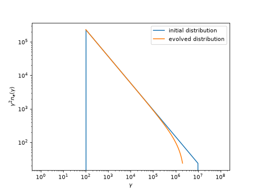
# let us plot both particle distributions, the initial and the evolved one
gamma = time_evolution_result.gamma
n_e_evol = time_evolution_result.density

fig, ax = plt.subplots()
n_e_initial.plot(ax=ax, gamma_power=2, label="initial distribution")
ax.plot(gamma, n_e_evol * gamma**2, label="evolved distribution")
ax.set_xlabel(r"$\gamma$")
ax.set_ylabel(r"$\gamma^2 n_e(\gamma)$")
ax.legend()
plt.show()

(Source code, png, hires.png, pdf)

As a side effect, the evaluate method replaces the internal electron distribution of the Blob with the newly calculated InterpolatedDistribution.

The TimeEvolution constructor accepts several optional parameters.

Parameters related to energy changes and particle injection:

energy_change_functions (mandatory)
rel_injection_functions
abs_injection_functions

Each of these parameters may be a single function or an array or a map of functions. During the time evolution, these functions are called at each time step and must return the energy change rates or injection rates as a Quantity. All of them accept a single parameter of class FnParams, containing three properties: gamma, an array of gamma (Lorentz factor) values; densities, a Quantity array of particle density values corresponding to the gamma array; and density_subgroups, a numpy array representing distribution of density values across density subgroups (see the section describing density groups). For the description of expected return values of each of these functions, see the pydoc of their respective types: EnergyChangeFn, InjectionRelFn and InjectionAbsFn

Parameters related to subinterval time calculation:

step_duration - time Quantity, or string “auto”
max_energy_change_per_interval - float
max_density_change_per_interval - float
max_injection_per_interval - float
optimize_recalculating_slow_rates - bool

These parameters define how the total evolution time is divided into smaller steps. The step_duration parameter may be set to a specific time, in which case the total evaluation time is split into equal steps of that duration. Alternatively, it can be set to the string “auto”, in which case each substep duration is computed automatically as the longest time interval that does not exceed the specified max_*_per_interval constraints. Additionally, setting optimize_recalculating_slow_rates to true instructs the algorithm to use longer time steps for bins with smaller change rates.

For example, setting step_duration=”auto” and max_density_change_per_interval=2.0 selects the longest time interval during which the electron density in each energy bin does not change by more than a factor of two.

Parameters related to bin management:

initial_gamma_array - 1D numpy array
gamma_bounds - Tuple[float, float]
max_bin_creep_from_bounds - float
merge_bins_closer_than - float

The time evolution logic divides the full energy spectrum (gamma values) into narrow bins and tracks the evolution of the energy and particle density in each bin.

Initial bins for the calculation are generated automatically, using the max/min gamma values of the ParticleDistribution of the Blob. You may, however, specify the initial bins explicitly using initial_gamma_array. Additionally, by setting gamma_bounds, any bins which have shifted beyond these bounds will remove from further calculations. Furthermore, two bins are merged when they become sufficiently close over time (controlled by merge_bins_closer_than). Additional bins are created at the lower or upper bounds if the lowest or highest bin drifts too far from the bounds (as defined by gamma_bounds with max_bin_creep_from_bounds).

Groups:

subgroups - list of lists of strings
subgroups_initial_density - 2D numpy array

Subgroups (also called just groups) allow the virtual splitting of the blob’s particle distribution into two or more subgroups, enabling different energy change and injection functions to be applied to each subgroup.

When using groups, the energy_change_functions, rel_injection_functions, and abs_injection_functions must be specified as maps (dictionaries) rather than arrays. The dictionary keys correspond to group names, which must be referenced as a list in the subgroups parameter to define which functions apply to which group.

The optional subgroups_initial_density parameter specifies the initial particle distribution across subgroups. If not provided, all particles over all energies are assigned to the first subgroup. If provided, it must be a 2D numpy array, with one dimension matching the subgroups length, and the other matching the initial_gamma_array length (initial gamma array is mandatory in this case).

Here is an example configuration with two subgroups. Synchrotron losses apply to both groups, acceleration applies only to the first group, and particle escape from the first group to the second is also configured:

TimeEvolution(
  blob,
  total_time,
  initial_gamma_array=gamma_array,
  energy_change_functions={"Synch": synchrotron_loss(synch), "Acc": fermi_acceleration(tacc)},
  rel_injection_functions={"Gr1-esc": escape_group1},
  abs_injection_functions={"Gr2-inj": injection_group2},
  subgroups=[["Synch", "Acc", "Gr1-esc"],
             ["Synch", "Gr2-inj"]]
)

Note: the escape_group1 and injection_group2 functions are user-defined and are not provided by agnpy. To correctly model particle escape from group 1 to group 2, the values returned by these functions must be synchronized.

For example, escape_group1 may assume that, over one second, half of the particles escape from group 1 (hence the use of a relative injection function). To maintain consistency, injection_group2 must convert this escaped fraction into an absolute injection rate for group 2 and apply the appropriate sign convention (negative values indicate particle loss).

Additional parameters:

method
distribution_change_callback

The method parameter allows switching from the default Euler method to the more accurate, but slower, Heun method. The distribution_change_callback parameter accepts a user-defined function that is called after each time step and can be used to track the progress of the calculation.

Energy change functions

The TimeEvolution class implements a generic algorithm for tracking changes in the particle energy spectrum. The algorithm itself is independent of any specific physical energy loss or gain process. It only requires one or more functions that take a gamma array as input and return the corresponding energy change rates.

These functions may be called multiple times during the evolution. Negative return values indicate energy loss, while positive values indicate energy gain.

The agnpy.time_evolution module provides four ready-to-use implementations:

synchrotron_loss - for Synchrotron energy losses in the magnetic field of the blob (used with a Synchrotron object);
ssc_loss - for IC losses on synchrotron photons in SSC process, including possible Klein-Nishina suppression (used with a SynchrotronSelfCompton object);
ssc_thomson_limit_loss - simplified, faster formula for IC losses, valid in the Thomson limit, without Klein-Nishina suppression;
fermi_acceleration - for simple Fermi-acceleration modelling.

Among these, ssc_loss is by far the most computationally expensive. When the Thomson limit is applicable, using ssc_thomson_limit_loss is strongly recommended for improved performance.